Enron : Catching the criminals with Data Science
In this project we look at all the public data made available on Enron, at one time one of the nations ten largest companies.
At Enrons peak it's shares were selling at \$90.75. In December of 2002, it was closing at \$0.27 .
In this paper we investigate Enron to see if we can identify known Persons Of Interest ( POI ) discovered during the governments investigation, through data including financial information like salary, bonus(es) and total_stock_values, as well as emails sent between members of the company.
We will step through the process of identifying , scaling and selecting features as well as training several classifiers such as GuassianNB, AdaBoost and DecisionClassifierTrees. Then we will use GridSearchCV to programatically tune each parameter to the classification pipeline and choose the best classifier based on a set of acceptance criteria, namely getting precision and recall scores above 30% , and accuracy above 80% .
The Data
Our journey into the Enron data starts with Exploratory Data Analysis ( EDA ). Our first task is to just look at the data and get an idea of the columns ( or features ) , missing data and outliers.
Persons of Interest
Our task in this project is to try and identify POI's, discovered during the trial, from only the raw enron data. Our project is a bit unique in that we have only 18 total persons of interest in a dataset with only 146 total entries, much smaller than datasets we've seen in the past. This will affect our outlier selection, as well as cross validation choice as we will see .
Missing Data
We have 146 total examples and 23 attributes after including full_name as a column as well as the index. After looking at some summaries created with Pandas , we notice some attributes have a lot of rows with missing values. These columns include director_fees ( missing 129 ) , loan_advances ( 142 ), restricted_stock_deferred ( 128 ) , deferral_payments ( 107 ).
After running a simple GuassianNB before and after removing those features, we see an increase in recall and precission right away.
Outliers
Let's take a look at our data to see if we notice anything obvious. The graphs below were created with RapidMiner Studio but could just as easily produced in python using matplotlib and a scatter plot.
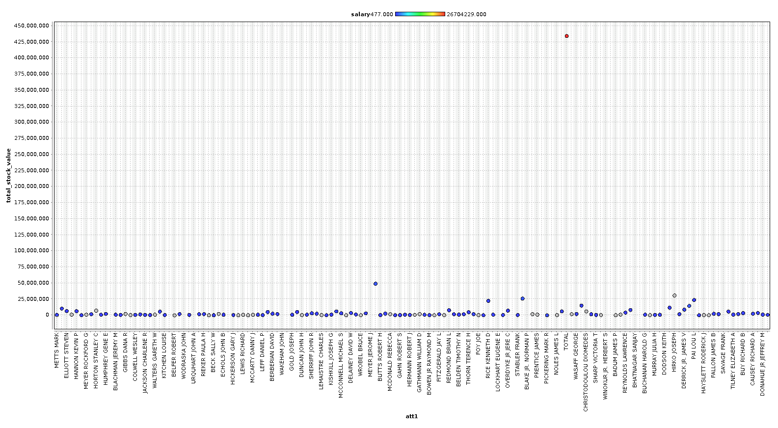
In the first initial round of plotting the data, we immediately notice one large outlier in ALL of the charts. It turns out that there was a TOTAL row that was totaling all of the data. Let's remove this entire row and plot again.
First let's look at the salary scatter plot.
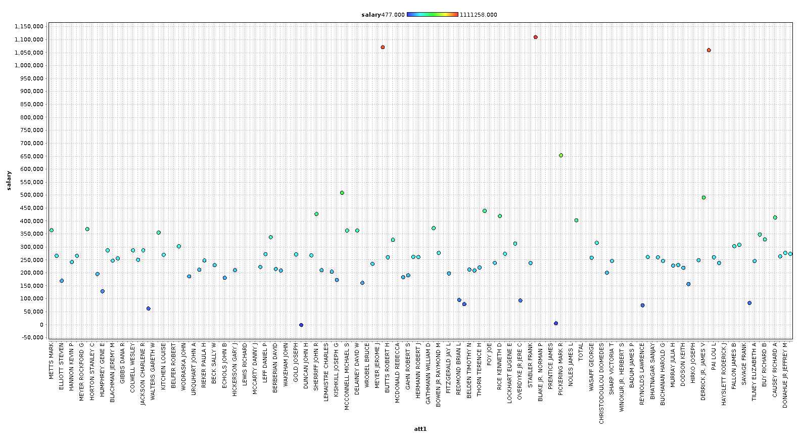
In this splot we are coloring the dots with salary, and we will color all subsequent charts with salary as well, to get a feel how bonus, stocks, and other financial features relate to our base 'salary' features.
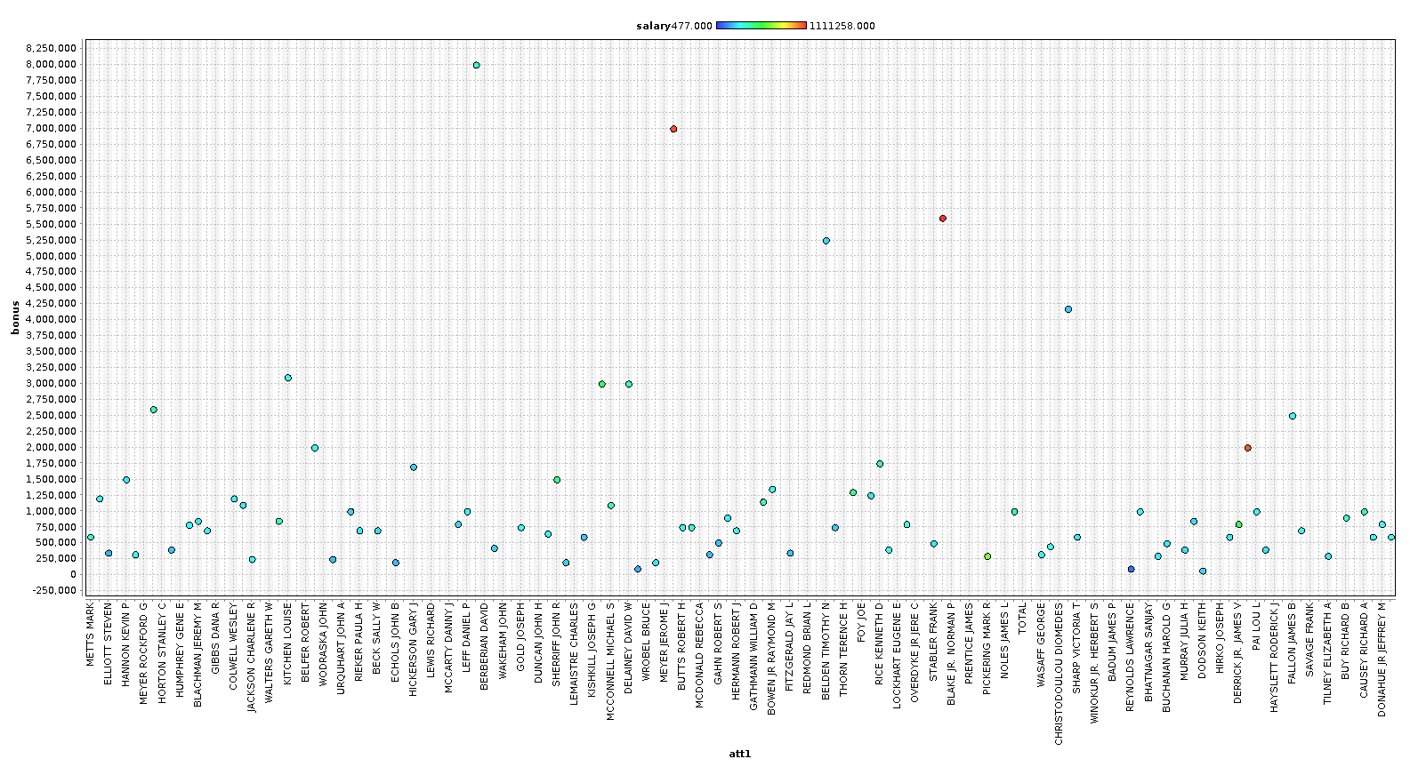
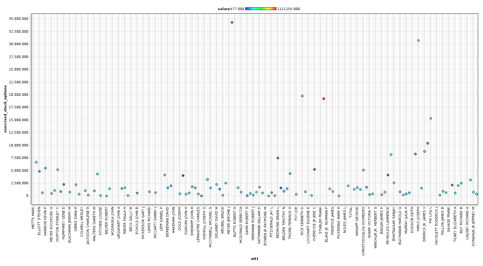
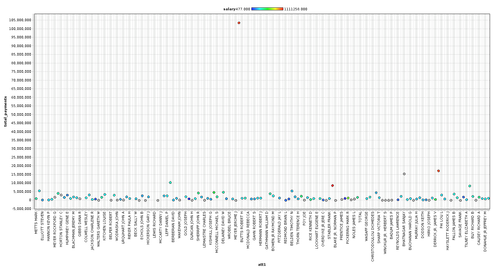
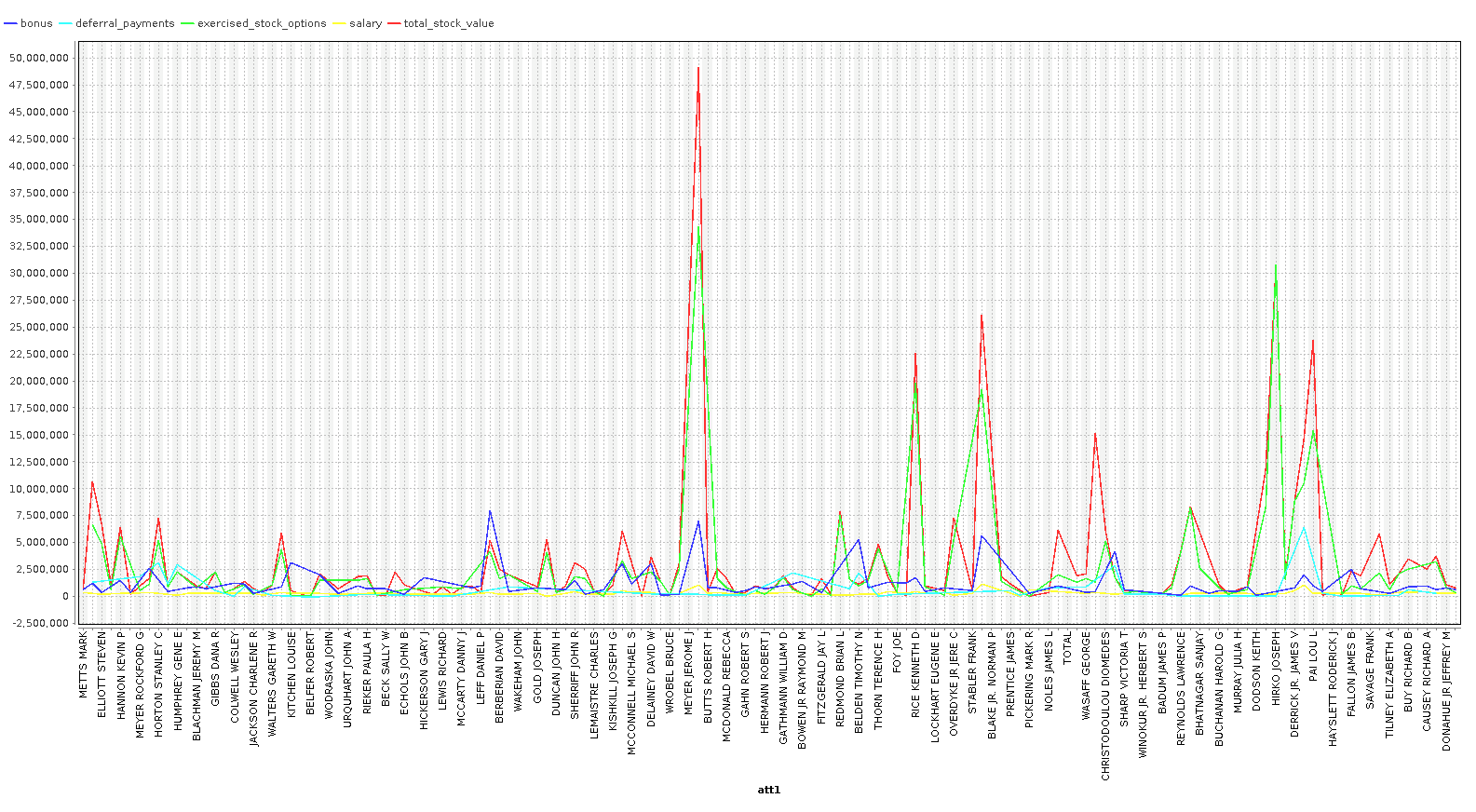
As you can see, we can identify some people that are clearly outliers in our data. In the last chart, we plot a line chart with several features and see a very clear pattern. In our case however, with only 146 examples, we are going to keep most the outliers, because these outliers are exactly the sort of data we are looking for. We are going to remove the columns ['director_fees', 'loan_advances', 'restricted_stock_deferred', 'deferral_payments'] , because they contain more rows with missing data than without.
Feature Generation
My initial GuassianNB implementation was only able to get around 25% accuracy, it wasn't until I added additional features detailing the interactions between possible POI's that I was able to get a better result. For our feature generation, we create new variables to_poi_score and from_poi_score, representing the amount of interaction to persons of interest, as well as from persons of interest. In the end , only our to score wound up adding predictive power to our classifier, so we only included one extra feature in the final implementation.
Feature Selection and Scaling
In the end , we ended up with 7 total features for testing with, ['poi','bonus','to_poi_score','salary','exercised_stock_options','total_stock_value','restricted_stock'] . Of these, our SelectAtMostKBest feature selector will further reduce this to only the features that are best at predicting our POI.
Scaling
For scaling our features, which we do both to speed up training and to get better accuraccy ( through the ability to run more permutations! ), we used sklearns StandardScaler. Below we have outputs of features_train for both before and after scaling.
# Before
    [[       0.        0.        0.   343434.   343434.        0.]
     [       0.        0.   130724.  2282768.  2282768.        0.]]
# After
    [[-0.5441382       0.    -1.06648677 -0.38168873 -0.4330838  -0.49781674]
     [-0.5441382       0.    -0.33467154 -0.01756374 -0.13748452 -0.49781674]]
Feature Selection
For feature selection, we are using two options chained in the pipline.
PCA
The first is Principal Component Analysis ( PCA ) , used to reduce our feature set to those features that have the most predictive power. PCA works by fitting an N dimensional space onto an N-1 dimensional space while trying to maintain the most variance. This is quite useful in ML when we have many features that might be similarly related, and using PCA can reduce our features from say 30 to 10 which we can use in our final predictors. In our project, our GridSearchCV will tune our parameters and find the best number of dimensions to work with, and it repeatedly came out with either 5 dimensions, or 4 dimensions, depending on the classifier being used.
Select K Best
SelectAtMostKBest , which is our own version of SelectKBest that works better with unbounded maximums, works by scoring each feature for its predictive power, than selecting at most K of these. In our GridSearch, we try several K's to see which one gives us the best predictive results, and choose only the K best that improve our predictive power. In this project, K was consistently at 4 or 2.
pipe = make_pipeline(StandardScaler(), PCA(n_components=len(features_list) - 1),
                             SelectAtMostKBest(k=len(features_list) - 1), c)
Classifiers
Our classifiers we chose to evaluate are DecisionTreeClassifier, GaussianNB, MLPClassifier, and AdaBoostClassifier. We will collect each of these in a list and iterate over it to collect the best scores from each. The final scores are in the final chart.
Training and Tuning the Classifiers
This authors approach uses a Pipeline ( for feature selection ) with a GridSearchCV ( for parameter tuning ) to find the best estimator. Our process looks something like
Input_Features -> Scale() -> Reduce_Features() -> Select_Best_Features() -> Classify() -> Test -> Repeat()
We then combine this with a list of parameters to each step , for example :
{
        "selectatmostkbest__k": range(1, len(features_list) - 1, 1),
        "pca__n_components": range(1, len(features_list) - 1, 1),
        "adaboostclassifier__learning_rate": [0.1, 1, 10],
        "adaboostclassifier__algorithm": ['SAMME', 'SAMME.R']
}
These parameters would be used with the AdaBoostClassifier specifiyng a list of parameters to its consturctor. In this example we are speciying a learning_rate of 0.1, 1 and 10, and an algorithm of 'SAMME' or 'SAMME.R'. The GridSearchCV we will be using will try every combination of these parameters and report back the best Estimator in bestestimator\, and the best score in bestscore\.
This would then be combined with score target ( we will be scoring both 'recall' and 'precission' to find the best Estimator ) , and our CrossValidation strategy which we will talk about in a later section.
All together it looks like
        pipe = make_pipeline(StandardScaler(), PCA(n_components=len(features_list) - 1),
                             SelectAtMostKBest(k=len(features_list) - 1), clf )
        search = GridSearchCV(pipe, params, cv=StratifiedShuffleSplit(), scoring=score, n_jobs=-1)
        search.fit(features_train, labels_train)
where clf is a variable containg either ( GuassianNB, DecisionTreeClassifier, MLPClassifier or ADABoosClassifier ) and score is either 'recal' or 'precision'. We specify n_jobs=-1 to tell sklearn to multi thread it unbounded.
GridSearchCV feature tuning and parameter selection results:
import pandas as pd
import numpy as np
import qgrid

df = pd.DataFrame(
    data=[[
        'DecisionTreeClassifier',
        " {'decisiontreeclassifier__presort': True, 'pca__n_components': 5, 'selectatmostkbest__k': 2, 'decisiontreeclassifier__criterion': 'entropy', 'decisiontreeclassifier__splitter': 'best'}",
        0.29950, 0.26634, 0.28195, 0.28195,  0.29222
    ], [
        'GaussianNB', "{'pca__n_components': 2, 'selectatmostkbest__k': 2}",
        0.48327, 0.32500, 0.85393, 0.38864, 0.34778
    ], [
        'MLPClassifier',
        "{'mlpclassifier__hidden_layer_sizes': (5, 5), 'pca__n_components': 5, 'selectatmostkbest__k': 4}",
        np.nan,
        np.nan
    ], [
        'AdaBoostClassifier',
        " {'adaboostclassifier__algorithm': 'SAMME.R', 'selectatmostkbest__k': 2, 'pca__n_components': 4, 'adaboostclassifier__learning_rate': 1}",
        0.27841, 0.23150, 0.80450,  0.25280, 0.23957
    ]],
    columns=[
        "Classifier", "Best Configuration", "Recall", "Precision", "Accuracy","F1", "F2"
    ],
    index=None)

pd.set_option('display.max_rows', len(df))
pd.set_option('display.max_colwidth', -1)
df
Evaluation and Validation
Validation and testing is a critical part of any Machine Learning application. In a typical scenario for supervised learning, we receive a set of data that has been classified or 'labeled' so that we can feed the classifier examples and 'teach' it our expected response from our input. In this scenario, we would split our data up into three parts, a training set - which we will use to train our classifiers on, a validation set , which we will use to validate our training on, and finally a testing set, a set of data that is not part of any training or validation processes so that we can ensure that the the metrics for our validation are clean and have not been altered by any training or validation. These metrics we will use for our evaluation of our classifiers, where we will evaluate and choose the classifier with the best predictive metrics.
Two import metrics we use in evaluation are precision and recall. Both of these can be thought of as measures of relevancy. Precision is measured as the ratio of retrieved documents from ones that are relevant, and recall is measured as a ratio of relevant documents that have been retrieved.
For our validation we are using a CrossValidation technique called StratifiedShuffleSplit ,which shuffles and samples our feature data by taking slices from various parts of the array (stratisfy). The Classifiers above are then fit 3 times (the default number of splits to StratifiedShuffleSplit ) with various testing from the strata and the best combinations of parameters are selected from the GridSearchCV , per classifier. We need to do this for each classifier we want, recording the scores and 'pickling' each one to then test again with tester.py , the standard testing agent.
Our MLPClassifier hit a 'divide by zero' exception right away and got eliminated. From the others, you can see that the GuassianNB has the best results for Recall, Precision, and Accuracy , with PCA N=2 and K=2 for features selection. That's 85% accuracy from our Naive Bayes classifier which indeed wins the entire contest.
And a note on the AdaBoostClassifier, it took 4 to 5 times longer to train and then again to test than the others and provided the least favorable results.
Final Results
In this project we developed a complete data science pipeline, from reading the data all the way to classification. We used StandardScaler to handle feature scaling for molding our data into an easily computable reudced form. We used PCA to reduce the dimensions or 'features' by eliminating those with the least variance, together with SelectAtMostKBest to select the K best features of that reduction.
Finally we used this Pipeline framework to train each of our classifiers in turn, testing sklearns GuassianNB, DecisionClassifier and AdaBoostClassifier, recording both the recall and precision, as well as F1 and F2 scores, of each classifiers "Best Estimator", which was found by using a GridSearchCV to tune parameters for each classifier.
We then use a CrossValidation technique called StratifiedShuffleSplit in order to validate and measure our classifiers. We chose this validation technique mainly because the little amount of data we had. By using shuffled parts of data, picked at random through out the entire training set, we can maximize the amount of training we can get out of our low volumne data.
In the end, the Guassian Naive Bayes classifier had the best results with 85% Accuracy, 48% Recall and 32% Precission in predicting our Persons of Interest.
References
I hereby confirm that this submission is my work. I have cited above the origins of any parts of the submission that were taken from Websites, books, forums, blog posts, github repositories, etc.
- New York Times, http://www.nytimes.com/2001/11/29/business/enron-s-collapse-the-overview-enron-collapses-as-suitor-cancels-plans-for-merger.html
- Wall Street Journal, https://www.wsj.com/articles/SB1007430606576970600
- NPR, http://www.npr.org/news/specials/enron/
- Wikipedia, https://en.wikipedia.org/wiki/Enron_scandal